Package architecture
Here we describe the various abstractions used to allow great flexibility in
the peri package while also allowing for a generalized framework for
optimization image updates (frequently through local updates and caching). The
description will proceed in three stages:
- The State – We talk about the
Stateclass, its properties, and model updates, through an example of fitting a polynomial. - The ImageState – We talk about the
ImageStateclass, its properties, and model updates, through an example of an image of Gaussian discs. - Optimization and Advanced Components – We talk about optimization of stage two, demonstrating the local update framework and other advanced components, through the optimization and model fitting of the image of Gaussian discs.
States (Example: PolyFitState)
In this section (with PolyFitState example), we will have noisy data which we wish to fit with a polynomial. While a relatively simple problem, we will implement it in the PERI framework, including how to get the best performance using various aspects of the package.
Overview
The basic structure needed to fit a model to data is the
State object. This structure holds the data and model and
provides a common interface that allows the peri package to optimize a set
of parameters to match the two. All of the common operations are implemented
(including but not limited to Jacobians, Hessians, log-likelihood, priors),
leaving you to implement only a few methods in order to have a functioning
State. In order to implement a
State, you must know about the following class methods:
-
class
peri.states.State(params, values, logpriors=None, hyper_params=[‘sigma’], hyper_values=[0.04], **kwargs) A model and corresponding functions to perform a fit to data using a variety of optimization routines. A model takes parameters and values (names and values) which determine the output of a model, which is then compared with data.
Parameters: - params (list of strings) – The names of the parameters (should be a unique set)
- values (list of numbers) – The corresponding values of the parameters
- logpriors (list of peri.prior.Prior) – Priors (constraints) to apply to parameters
- hyper_params (list of strings, optional) – The names of any hyper-parameters (should be a unique set). Stored as a peri.comp.ParameterGroup. Default is [‘sigma’], the standard-deviation of the noise distribution.
- hyper_values (list of numbers, optional) – The corresponding values of the hyper-parameters. Stored as a peri.comp.ParameterGroup. Default is [0.04]
- kwargs – Arguments to pass to super class
peri.comp.ParameterGroupincluding ordered and category.
-
data Class property – the raw data of the model fit. Should return a number (preferrably float) or an ndarray (essentially any object which as operands +-/…). This object is constant since it is data.
-
model Class property – the current model fit to the data. Should return a number or ndarray. Ideally this object should be an object updated by the
peri.states.State.update()function and simply returned in this property
-
update(params, values) Update a single parameter or group of parameters
paramswithvalues.Parameters: - params (string or list of strings) – Parameter names which to update
- value (number or list of numbers) – Values of those parameters which to update
State class
To demonstrate this State class, let’s implement a polynomial fit class
which fits a one dimensional curve to an arbitrary degree polynomial. In the
following class, we subclass State and implement the
properties and functions that we outlined in the previous section. In
particular, in the __init__, we store the input x points as a member
variable and y values as data. We then set up parameter names and values
depending on whether the user supplied coefficients the init. We call the
superclasses’ init and call update with these parameters and values to make
sure that the model is calculated.
import numpy as np

class PolyFitState(peri.states.State):
    def __init__(self, x, y, order=2, coeffs=None):
        self._data = y
        self._xpts = x

        params = ['c-%i' %i for i in xrange(order)]  # names for the coefficients
        values = coeffs if coeffs is not None else [0.0]*order  # and their values

        super(PolyFitState, self).__init__(
            params=params, values=values, ordered=False
        )

        self.update(self.params, self.values)

    def update(self, params, values):
        super(PolyFitState, self).update(params, values)
        self._model = np.polyval(self.values, self._xpts)

    @property
    def data(self):
        return self._data

    @property
    def model(self):
        return self._model
The update function for this class simply uses numpy’s polyval function
to evaluate the parameter values as a polynomial at the stored x values.
This model value is stored as a member variable and returned for the model
property. The data property is simple the stored y values.
We can then make an instance of this PolyFitState and begin to fit fake
‘data’ with our model.
# noise level
sigma = 0.3

# num of coefficients, datapoints
C, N = 8, 1000

# generate data
np.random.seed(159)
c = 2*np.random.rand(C) - 1
x = np.linspace(0.0, 2.0, N)
y = np.polyval(c, x) + sigma*np.random.randn(N)

# create a state
s = PolyFitState(x, y, order=C)
Properties
We can check out some of the common functions provided to State objects
before we begin to optimize. For example, we can look at an approximation to
the sensitivity matrix \(J^T J\):
import matplotlib.pyplot as pl
pl.imshow(s.JTJ(), cmap='bone')
pl.xticks(np.arange(len(s.params)), s.params)
pl.yticks(np.arange(len(s.params)), s.params)
pl.title(r"$J^T J$ for PolyFitState")
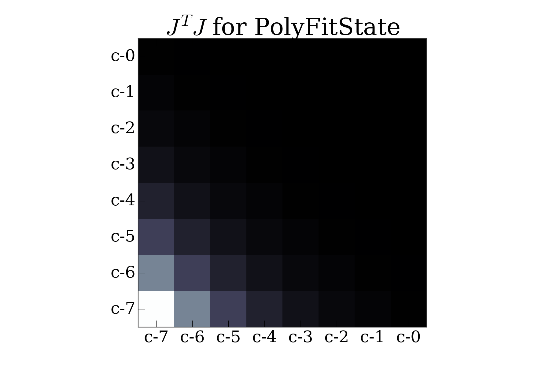
Showing the relatively boring structure of \(J^T J\) for the PolyFitState.
or we can calculate the Cramer-Rao bound for the fit parameters:
s.crb()
Optimization
From here, we can optimize the parameters of the state along with the estimated
noise level. peri provides several ways to optimize the state’s parameters.
First, we will demonstrate using Monte Carlo sampling, particularly with
a multidimensional slice sampler, to optimize the state:
from peri.mc import sample

# burn a number of samples if hadn't optimized yet
#h = sample.sample_state(s, s.params, N=1000, doprint=True, procedure='uniform')

# then collect the samples around the true value
h = sample.sample_state(s, s.params, N=30, doprint=True, procedure='uniform')

# distribution of fit parameter values
h.get_histogram()
We can also optimize the PolyFitState using variations on nonlinear least
squares optimization with Levenberg-Marquardt.
import matplotlib.pyplot as pl
import peri.opt.optimize as opt
opt.do_levmarq(s, s.params[1:])

fig = pl.figure()
pl.plot(s._xpts, s.data, 'o', label='Data')
pl.plot(s._xpts, s.model, '-', label='Model')
pl.xlabel(r"$x$")
pl.ylabel(r"$y$")
pl.legend(loc='best')
pl.title("Best fit model")
![``opt.do_levmarq(s, s.params[1:]); pl.plot(s.data); pl.plot(s.model)``](_images/arch_polyfit_fit.png)
Comparison of data and model fit for PolyFitState with data seeded from an 8th order polynomial with noise.
All the code listed above can be downloaded here.
Image states (Example: GaussianDiscModel)
Since a common usage pattern of PERI is to optimize models of experimental
microscope images, we implemented a very flexible ImageState which
provides:
- Easy implementation of new model equations
- Compartmentalization of parts of an image
- Many optimizations including local image updates and better FFTs
On top of the State class, we add several layers of
complexity. We feel these levels of complexity help, rather than hinder, the
development of new image models and allows the flexibility to adapt to new
brands and types of microscopes and experimental systems. Here we will describe
these structures and along the way develop a very simple image model of
polydisperse discs in a plane imaged with microscope described by a Gaussian
point-spread-function (PSF). In particular, the model we will be creating is:
where \(P\) is the point spread function and \(S\) is the shape function which defines the Platonic solid, and \(B\) is a spatially varying background which may represent any number of confounding factors in image formation. We’ll start with a simple model of two-dimensional circular discs, infludenced by microscope optics through an anisotropic Gaussian point- spread function, and imaged on a detector with non-uniform background:
Since each of this functional form seem distinct, we separate our model into
small objects which we call components. These components calculate part
of the model (\(P\), \(S\), …) over a certain region, or Tile,
then get combined back into the overall model. This philosophy can be expressed
simply as:
- Model (
Model) – The entire equation (and derivatives) describing the image formation \(\mathcal{M}\) - Component (
Component) – Small subsections of the model e.g. \(P\), \(S\), \(B\) - Tile (
Tile) – Regions of the image over which parts of the model are calculated.
Model
We will start our description from the top down, first describing the
Model, or the equation that produces our model image. To create a new model,
we simply subclass the Model class and overwrite the
__init__ function. This function holds the actual equations which are
called to calculate the model image. For our example here, let’s simply
translate the equation above:
import peri.models

class GaussianDiscModel(peri.models.Model):
    def __init__(self):
        # gives human readable labels to equation variables
        varmap = {'P': 'psf', 'D': 'disc', 'C': 'off'}

        # gives the full model equation of applying the psf P to an image
        # of discs D and adding an offset because the peak-to-peak of
        # real images is often hard to discern
        modelstr = {'full' : 'P(D) + C'}

        # calls the super-class' init
        super(GaussianDiscModel, self).__init__(
            modelstr=modelstr, varmap=varmap, registry=None
        )
As mentioned in the comments for the code segment, we first have a varmap
(variable map) that essentially acts to give human labels to the variables in
the model equation. We define a psf \(P\), disc image \(D\), and
constant offset \(C\). The modelstr defines the actual equation (which
will be eval’d) in terms of the variables defined above. In this equation,
the Component given by each label (psf, disc, off) will have their
get() function called and inserted into the string. More on this later.
We are done with this section of the example. In the next example we will talk
about necessary optimizations to include to make this Model perform better.
Components
The items that we listed in the model (psf, disc, off) must be a subclass of
Component or
ComponentCollection. These objects are essentially a
group of parameters and values (names and numbers), knowledge of how to compute
something, and a method to update itself. They can be significantly more
complicated depending on various optimizations, but we will here demonstrate
the most basic form of a Component (we will get complicated in the next
example).
ParameterGroup
At the lowest level, a Component is a ParameterGroup, a storage
container for values and names associated with those values. A
ParameterGroup is a container that provides a common
interface to any object which computes “something” based on a set of
parameters (string names) and values (the values associated with those
names). In the most basic form, a ParameterGroup must care about the
following structure:
-
class
peri.comp.comp.ParameterGroup(params=None, values=None, ordered=True, category=’param’) Any object which computes something based on parameters and values can be considered a
ParameterGroup. This class provides a common interface sinceParameterGroupappears throughoutPERIincludingComponents,Priors,States. In the very basic form, aParameterGroupis adictorOrderedDictof:{ parameter_name: parameter_value, ... }
The use of a dictionary is strictly optional – as long as the following methods are provided, the parameters and values may be stored in any format that is convenient:
Parameters: - params (string, list of strings) – The names of the parameters, in the proper order
- values (number, list of numbers) – The values corresponding to the parameter names
- ordered (boolean (default: True)) – If True, uses an OrderedDict so that parameter order is deterministic independent of number of parameters
- category (string (default: 'param')) –
Name of the category associated with this ParameterGroup.
Warning
FIXME : should only be a property of Component
-
get_values(params) Get the value of a list or single parameter.
Parameters: params (string, list of string) – name of parameters which to retrieve
-
set_values(params, values) Directly set the values corresponding to certain parameters. This does not necessarily trigger and update of the calculation,
See also
update(): full update func
-
update(params, values) Update the calculation of the class based on a pair or pairs of parameters and associated values.
Parameters: - params (string, list of strings) – name of parameters to update
- values (number, list of numbers) – cooresponding values to update
In order to implement a Component, you should be familiar with the methods
listed above.
Component
A subclass of the ParameterGroup is a Component which is a group of
values which are used to compute part of the model image. Therefore, its
update() function must actually update the necessary parts of the
computation for that component. Additionally, the Components must know
something about the dimensions of the image over which they are expected to
function as well as the current area of interest. It must also provide
information about which parts of the image it finds important (but won’t deal
with this until the next section). Therefore, in the Component
class we need to know about:
-
class
peri.comp.comp.Component(params, values, ordered=True, category=’comp’) A
ParameterGroupwhich specifically computes over sections of an image for anImageState. To this end, we require the implementation of several new member functions:In order to facilitate optimizations such as caching and local updates, we must incorporate tiling in this object.
Parameters: - params (string, list of strings) – The names of the parameters, in the proper order
- values (number, list of numbers) – The values corresponding to the parameter names
- ordered (boolean (default: True)) – If True, uses an OrderedDict so that parameter order is deterministic independent of number of parameters
- category (string (default: 'param')) – Name of the category associated with this ParameterGroup.
-
get() Return the natural part of the model. In the case of most elements it is the calculated field, for others it is the object itself.
-
get_padding_size(tile) Get the amount of padding required for this object when calculating about a tile tile. Padding size is the total size, so half that on each side. For example, if this Component is a Gaussian point spread function, then the padding returned might be:
peri.util.Tile(np.ceil(2*self.sigma))
Parameters: tile ( Tile) – A tile defining the region of interestReturns: pad – A tile corresponding to the required padding size Return type: Tile
-
get_update_tile(params, values) This method returns a
Tileobject defining the region of a field that has to be modified by the update of (params, values). For example, if this Component is the point-spread-function, it might return a tile of entire image since every parameter affects the entire image:return self.shape
Parameters: - params (single param, list of params) – A single parameter or list of parameters to be updated
- values (single value, list of values) – The values corresponding to the params
Returns: tile – A tile corresponding to the image region
Return type:
-
initialize() Begin anew and initialize the component
-
set_shape(shape, inner) Set the overall shape of the calculation area. The total shape of that the calculation can possibly occupy, in pixels. The second, inner, is the region of interest within the image.
-
set_tile(tile) Set the currently active tile region for the calculation
The flow-chart below illustrates the hierarchy of class inheritance in
peri.

Inheritance flowchart for the peri package. Arrows indicate inheritance.
Let’s sink our teeth in and create 2 of the components that will work in our
GaussianDiscModel (one already available in the peri package). We will
first create something to use as the psf, then a component to use as the disc
element of the image. The offset component is already implemented in
GlobalScalar.
GaussianPSF
import peri.util
import peri.comp.comp
from peri.fft import fft, fftkwargs, fftnorm

import numpy as np

class GaussianPSF(peri.comp.comp.Component):
    def __init__(self, sigmas=(1.0, 1.0)):
        # setup the parameters and values which will be passed to super
        super(GaussianPSF, self).__init__(
            params=['psf-sx', 'psf-sy'], values=sigmas, category='psf'
        )

    def get(self):
        """
        Since we wish to use the GaussianPSF in the model by calling P(D), the
        get function will simply return this object and we will override
        __call__ so that we can use P(...).
        """
        return self

    def __call__(self, field):
        """
        Accept a field (numpy.ndarray), apply the point-spread-function,
        and return the resulting image of a blurred field
        """
        # in order to avoid translations from the psf, we must create
        # real-space vectors that are zero in the corner and go positive
        # in one direction and negative on the other side of the image
        tile = peri.util.Tile(field.shape)
        rx, ry = tile.kvectors(norm=1.0/tile.shape)

        # get the sigmas from ourselves
        sx, sy = self.values

        # calculate the real-space psf from the r-vectors and sigmas
        # normalize based on the calculated values, not the usual normalization
        psf = np.exp(-((rx/sx)**2 + (ry/sy)**2)/2)
        psf = psf / psf.sum()

        # perform the convolution with ffts and return the result
        out = fft.fftn(fft.ifftn(field)*fft.ifftn(psf))
        return fftnorm(np.real(out))

    def get_padding_size(self, tile):
        # claim that the necessary padding size for the convolution is
        # the size of the padding of the image itself for now
        return peri.util.Tile(self.inner.l)

    def get_update_tile(self, params, values):
        # if we update the psf params, we must update the entire image
        return self.shape
PlatonicDiscs
import peri.util
import peri.comp.comp
import numpy as np

class PlatonicDiscs(peri.comp.comp.Component):
    def __init__(self, positions, radii):
        comp = ['x', 'y', 'a']
        params, values = [], []

        # apply using naming scheme to the parameters associated with the
        # individual discs in the object pos and rad
        for i, (pos, rad) in enumerate(zip(positions, radii)):
            params.extend(['disc-{}-{}'.format(i, c) for c in comp])
            values.extend([pos[0], pos[1], rad])

        # use our super-class structure to keep track of these parameters
        self.N = len(positions)
        super(PlatonicDiscs, self).__init__(
            params=params, values=values, category='disc',
        )

    def draw_disc(self, rvec, i):
        # get the position and radii parameters cooresponding to this particle
        pparams = ['disc-{}-{}'.format(i, c) for c in ['x', 'y']]
        rparams = 'disc-{}-a'.format(i)

        # get the actual values of these parameters
        pos = np.array(self.get_values(pparams))
        rad = self.get_values(rparams)

        # draw the disc using the provided rvecs and now pos and rad
        dist = np.sqrt(((rvec - pos)**2).sum(axis=-1))
        return 1.0/(1.0 + np.exp(5.0*(dist-rad)))

    def get(self):
        # get the coordinates of all pixels in the image. however, make sure
        # that zero starts in the interior of the image where the padding stops
        rvec = self.shape.translate(-self.inner.l).coords(form='vector')

        # add up the images of many particles to get the platonic image
        self.image = np.array([
            self.draw_disc(rvec, i) for i in xrange(self.N)
        ]).sum(axis=0)

        # return the image in the current tile
        return self.image[self.tile.slicer]

    def get_update_tile(self, params, values):
        # for now, if we update a parameter update the entire image
        return self.shape
ImageState, fitting, and properties
Now that we have implemented an GaussianDiscModel along with various
compatible components, let’s create a valid ImageState and explore its
properties and perform a fit to fake data. First, we can create a state
by using the Model and Components that we just created:
def initialize():
    N = 32

    # create a NullImage, which means that the model image will be used for data
    img = peri.util.NullImage(shape=(N,N))

    # setup the initial conditions for the parameters of our model
    pos = [[10., 10.], [15., 18.], [8.0, 24.0]]
    rad = [5.0, 3.5, 2.2]
    sig = [2.0, 1.5]

    # make each of the components separately
    d = PlatonicDiscs(positions=pos, radii=rad)
    p = GaussianPSF(sigmas=sig)
    c = GlobalScalar(name='off', value=0.0)

    # join them with the model into a state
    s = peri.states.ImageState(img, [d, p, c], mdl=GaussianDiscModel(), pad=10)
    return s
Once we have created the state s, let’s look at some of its properties.
Many of them are the same as the properties available in the PolyFitState
example since they inherit from State. For example,
we can look at derivatives of the model w.r.t. different parameters using
the following convenience function:
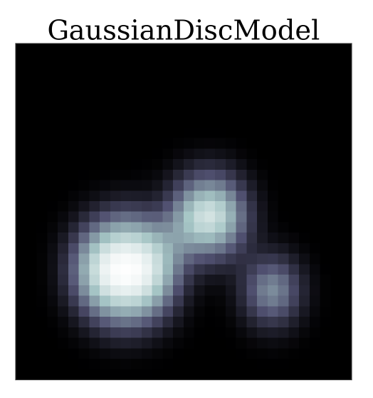
The model image create from our ImageState
Plotting the derivatives with respect to model parameters can be performed with
s.gradmodel:
def show_derivative(s, param, ax=None):
    # if there is no axis supplied, create a new one
    ax = ax or pl.figure().gca()

    # calculate the derivative of the model
    deriv = s.gradmodel(params=[param], flat=False)[0]

    # plot it in a sane manner using matplotlib
    scale = max(np.abs([deriv.min(), deriv.max()]))
    ax.imshow(deriv, vmin=-scale, vmax=scale, cmap='RdBu_r')
    ax.set_title(param)
    ax.set_xticks([])
    ax.set_yticks([])
This code yields the following images
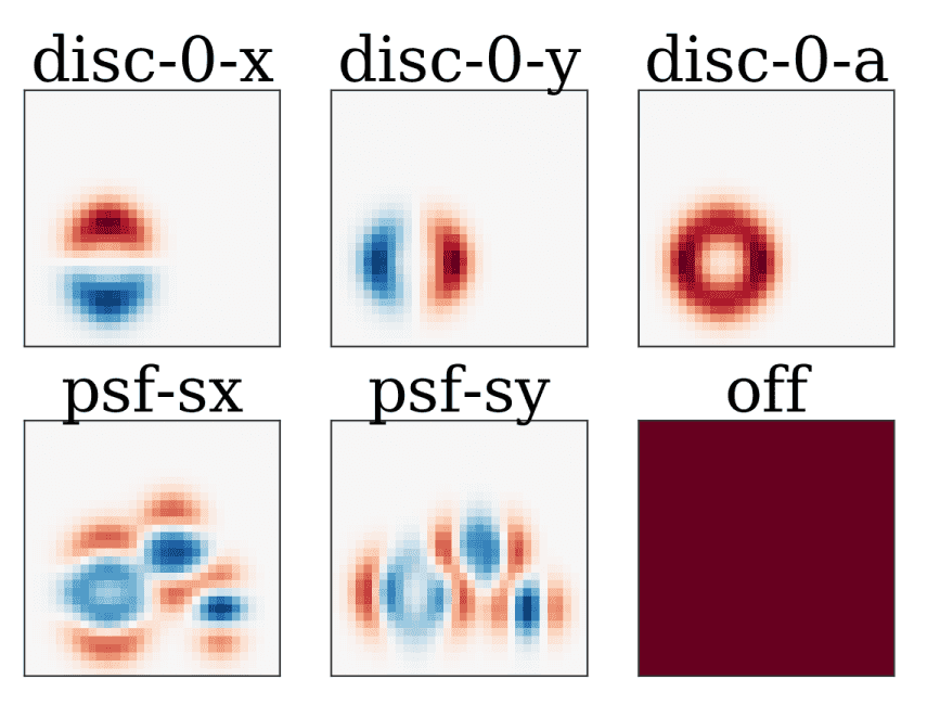
Gradients of the state with respect to various parameters in the model
Similarly, the \(J^T J\) can be plotted using the s.JTJ convenience
function
def show_jtj(s):
    # plot the JTJ with properly labeled axes
    p = s.params
    pl.imshow(np.log10(np.abs(s.JTJ())), cmap='bone')
    pl.xticks(np.arange(len(p)), p, rotation='vertical')
    pl.yticks(np.arange(len(p)), p, rotation='horizontal')
    pl.title(r'$J^T J$')
Yields the approximate hessian
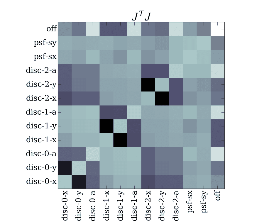
\(J^T J\) for the GaussianDiscModel with the components we created earlier in this section. You can see the strong coupling between neighboring particles as well as the coupling between global values (psf and off) and local ones (disc)
Finally, let’s make sure that our model is able to accurately reproduce the data (which happens to be generated from the model but has noise added to it). To do this, we will rattle the values of the model then perform a fit and compare the fit and errors to the true values.
def rattle_and_fit(s):
    # grab the original values
    values = np.array(s.values).copy()

    # update the model with random parameters then optimize back
    s.update(s.params, values + np.random.randn(len(values)))
    opt.do_levmarq(s, s.params, run_length=12)

    # calculate the crb for all parameters
    crb = s.crb()

    # print a table comparing inferred values
    print(' {:^6s} += {:^5s} | {:^8s}'.format('Fit', 'CRB', 'Actual'))
    print('-'*27)
    for v0, c, v1 in zip(s.values, crb, values):
        print('{:7.3f} += {:4.3f} | {:7.3f}'.format(v0, c, v1))
Running this function yields a table:
  Fit   +=  CRB  |  Actual
---------------------------
  9.964 += 0.026 |  10.000
 10.003 += 0.026 |  10.000
  5.023 += 0.019 |   5.000
 15.092 += 0.042 |  15.000
 17.910 += 0.038 |  18.000
  3.480 += 0.025 |   3.500
  7.995 += 0.056 |   8.000
 23.937 += 0.047 |  24.000
  2.198 += 0.024 |   2.200
  1.983 += 0.032 |   2.000
  1.515 += 0.034 |   1.500
  0.001 += 0.002 |   0.000
All the code listed above can be downloaded here.