PERI Walkthrough¶

What is PERI?¶

PERI is a general, methodological framework to extract the maximum amount of information from a single microscope image. The idea of PERI is simple and short:

Take a microscope image.
Create a mathematical model of the image formation process.
Fit that mathematical model to the image.
If the fit is not good, improve the mathematical model.
If the fit is good, use the extracted information from the fit.

The Python package peri contains both a general implementation of this framework and a detailed implementation of it for confocal images. In this walkthrough, I’ll show you how to use the Python peri package to start from an image and extract the maximal possible information from it. I’ll demonstrate this process on a real image from a confocal microscope, explaining each step along the way but trying to avoid getting mired in details. Finally, I’ll show you some convenience functions implemented in peri that make this process faster, both for you and your computer.

Before you begin, you’ll need to install peri. See the Installation section for how to do this.

Take a microscope image.¶

This is all you. A word to the wise though – analysis with peri takes time (step 3), and figuring out what the best mathematical model is (steps 2 and 4) takes even more time. You can save a lot of time by taking the cleanest possible data and avoiding as many imaging artifacts as possible, eliminating aspects of your image that are hard to model.

We’ll start by loading a small demo image with the package peri. First, download my test image. Then, open your Python interpreter and type:

from peri import util
im = util.RawImage('small_confocal_image.tif')

This creates an object which contains rescaled raw data and allows for small manipulations of the image by peri. If you’d like to look at the image interactively, you can use the OrthoViewer.

from peri.viz.interaction import OrthoViewer
OrthoViewer(im.get_image())

This will pull up an image like the one below, showing three orthogonal views of the three-dimensional tiffstack. Clicking on one of these will recenter the views on the region you clicked.

Create a mathematical model of the image formation process.¶

The method PERI needs a mathematical model to reconstruct the experimental image. At the grossest level, the model needs to create a model image. This model also needs to have parameters (e.g. the positions of the particles or the properties of the microscope) which are adjustable. PERI then fits those parameters to find the best-possible model of the experimental image.

In the package peri, the mathematical model itself is split into two parts: the components of the model, and the interaction between those components to create a final image. A component of the model is a description of a physical property of the sample or microscope – for instance, the distribution \(\Pi\) of fluorescent dye in the image or the intensity \(I\) of the light source. In addition, we need to know how these components interact mathematically to form a model image – e.g. the dye gets illuminated by the light as \(I\times \Pi\).

Let’s do a concrete example with our image above.

First, we need to figure out what components form our model.

Looking at the image, we see that the sample is composed of a coverslip slide and a lot of spheres. We can start by creating those objects with an initial guess for the particle positions and the following code:

import numpy
from peri.comp import objs
coverslip = objs.Slab(zpos=6)
particle_positions = numpy.load('particle-positions.npy')
particle_radii = 5.0  # a good guess for the particle radii, in pixels
particles = objs.PlatonicSpheresCollection(particle_positions, particle_radii)

All the model components in peri are stored in the module peri.comp. The components describing the microscope sample being imaged are stored in peri.comp.objs, which we import in the first line. In the next line, we create a coverslip, which is described by a peri.comp.objs.Slab object. Finally, in the last line we create a collection of spheres, described by peri.comp.objs.PlatonicSpheresCollection.

To speed up peri ‘s fit of the model, I’ve created both of these objects with reasonable initial guesses for the objects’ parameters. By looking at the raw image, I’ve seen that the coverslip is positioned at a height of roughly z=6 pixels above the bottom of the image. If I wanted, I could also pass a selection of Euler angles to describe the coverslip’s orientation. However, a flat coverslip is a good enough initial guess. Likewise, I’ve used a centroid algorithm (trackpy) to do a reasonable job finding most of the spheres in the image; the position guess for this is saved as 'particle-positions.npy' [1]. You can check the quality of this initial guess with the OrthoPrefeature, which overlays the image with the extracted particle positions:

from peri.viz.interaction import OrthoPrefeature
OrthoPrefeature(im.get_image(), particle_positions, viewrad=3.0)

``OrthoPrefeature(im.get_image(), particle_positions, viewrad=3.0)``

Click around to look at particles! If you like, you can add or remove particles by hitting A or R.

Clicking around shows that we’ve gotten most of the particles with our initial featuring, which is really all that peri needs to start. Finally, by looking at the raw data I’ve noticed that the particle radii are all about 5 pixels.

[1]	If and when you’re analyzing your own confocal images of spheres you can pass your initial guess for the positions as an [N,3] numpy.ndarray, which you can get however your heart desires, including through `locate_spheres()`.

Looking at the image, we see that the coverslip and particles behave the same way – both exclude dye from regions of the image. Thus, it seems best to treat these two objects together when we make our mathematical model, rather then separately. We can do this by grouping these two objects together:

from peri.comp import comp
objects = comp.ComponentCollection([particles, coverslip], category='obj')

A group of any model components is described by a peri.comp.ComponentCollection. Since we’ve collected these components together, we describe them (category='obj') so peri can identify to which part of the model they belong.

Next, we see that the image is illuminated by a laser, with stripe-like imperfections. We can create this object with this snippet:

from peri.comp import ilms
illumination = ilms.BarnesStreakLegPoly2P1D(npts=(16, 10, 8, 4), zorder=8)

Mathematically, we can describe the illumination as some sort of continuous field defined over the image. These field-like descriptions are stored in the module peri.comp.ilms, which we import in the first line. A quick look at the module shows that there are a sizeable number of possible illumination field descriptions. All of these conceptually do the same thing, but they are each parameterized slightly differently. After a lot of experimentation, I’ve found that the streaky-structure in my image is well-described by the technical-sounding BarnesStreakLegPoly2P1D [2]. In general, the different options in the ilms module are ways to parameterize the illumination, but they each need to know how many parameters to use. For my microscope, I’ve found that a good number of parameters for images of this size is what I’ve typed in – any less and the illumination isn’t described sufficiently, and more is overkill [3]. You will need to figure out how many parameters to include for your microscope and image size. For now, don’t worry about this – we’ll go over this in step 4.

[2]

Briefly, this consists of a series of Barnes interpolants in the x-direction, each multiplied by a different Legendre polynomial in the y-direction, to create a 2D field in x & y. The 2D field in x&y is then multiplied by a second Legendre polynomial in z to create an illumination that varies in three-dimensions. If you have a stripey illumination in the x-direction then this is the illumination for you. If not, then no worries – we discuss other options in the illumination section.

[3] If you want to know what these particular parameters mean – the tuple npts is the number of points for each Barnes interpolant in each direction; the size of the tuple sets the order of the Legendre polynomial in y. The int zorder is the order of the Legendre polynomial in z. You can see the documentation for details.

In addition, from knowing my microscope I know that (1) there is a background intensity always registered on the detector and (2) this background intensity actually varies with position. We can describe this spatially-varying background with the one-liner:

background = ilms.LegendrePoly2P1D(order=(7,2,2), category='bkg')

Since the background is just a spatially-varying field like the illumination, I’ve described it with another representation of a field from the ilms module. Here, the parameterization is as a 2D Legendre polynomial in x & y, and an additional Legendre polynomial in z. However, to allow peri to distinguish between the background and illumination components of the model, I’ve changed the category of the background to ‘bkg’ [4]. Finally, I’ve set the order (number of parameters in the Legendre polynomials) to numbers that I’ve empirically found work for me [5]. In addition, for numerical reasons we include an offset which takes into account high-frequency changes in the background. We do this with:

from peri.comp import comp
offset = comp.GlobalScalar(name='offset', value=0.)

[4]	All the model components have categories; for most of the rest the default category is good enough for me.

[5]	See the paper’s supplemental information for details on why the numbers are what they are, in particular why the z-order is so large.

Finally, I can see that the image is blurry, due to the wave-nature of light blurring out the image. We can describe this blurring with a point-spread function:

from peri.comp import exactpsf
point_spread_function = exactpsf.FixedSSChebLinePSF()

Representations of point-spread functions that use exact optical models are stored in the exactpsf module. I’ve chosen to describe my image with an optical model of a line-scanning point-spread function (the LinePSF bit), with some special numerical implementations made for speed and reliability (the FixedSSCheb bit). If you don’t want or need an exact optical description of your point-spread function, then you can use one of the heuristic functions stored in the module peri.comp.psfs (such as a Gaussian or a Gaussian that changes in z).

Now that we have all the components of the mathematical model, we need to describe how they interact. We do this by using the relationship for a confocal image:

from peri import models
model = models.ConfocalImageModel()

The model tells peri how to combine all the objects together to create an image. Our ConfocalImageModel knows that the objects in the sample excludes dye from certain regions, the dye gets illuminated by a laser, blurred by the point-spread function with microscope optics, and imaged on a detector with a spatially-varying background. You can see what this model mathematically is by typing

print model

Finally, we need to combine the mathematical model and its components together to create a model image. In peri, the image, the mathematical model, its parameters and values, and the model image are all stored in an object called a State or ImageState. We’re now ready to create our state:

from peri import states
st = states.ImageState(im, [objects, illumination, background,
        point_spread_function, offset], mdl=model)

If we want to save our state or load a saved state, we can use peri.states.save() and peri.states.load(). Finally, peri allows the same parameter to describe multiple components of the model. For instance, physically we know that the ratio of the z-pixel to xy-pixel size is the same whether we’re calculating an optical model of the point-spread function or drawing the Platonic particles. We can link these parameters with

from peri import runner
runner.link_zscale(st)

Fit that mathematical model to the image.¶

Our state contains information about the quality of the fit through the difference between the model and the image through two main attributes: st.residuals, which returns the difference between the model image and the experimental image, and st.error, which returns the sum of the squares of the residuals. Look at the error by typing

print st.error

Right now the fit’s error is pretty bad. We can fit the state and improve the error significantly using the convenience functions in peri.runner:

from peri import runner
runner.optimize_from_initial(st)

This fits the state, printing information to your screen and saving progress to your current directory along the way. If running this code doesn’t fit the state well enough, you can either re-run the code above again, or run:

runner.finish_state(st)

For a typical image, peri needs to fit thousands of parameters in a complex landscape, which can take a lot of time. Be patient. Or better yet, leave your computer and come back after lunch or tomorrow. If the convenience functions don’t work well for you or you want to delve into more details of the optimization methods, you can read about them in the documentation’s Optimization section, including how peri can automatically add missing particles and remove bad ones.

If the fit is not good, improve the mathematical model.¶

Now that we’ve fit our data, we need to check if the fit is good. peri provides several ways to do this for a single state. The first step is the OrthoManipulator:

from peri.viz.interaction import OrthoManipulator
OrthoManipulator(st)

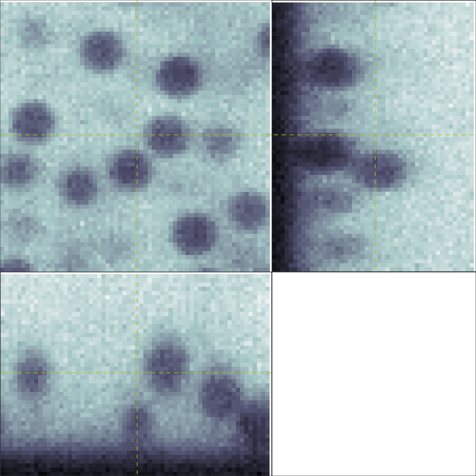
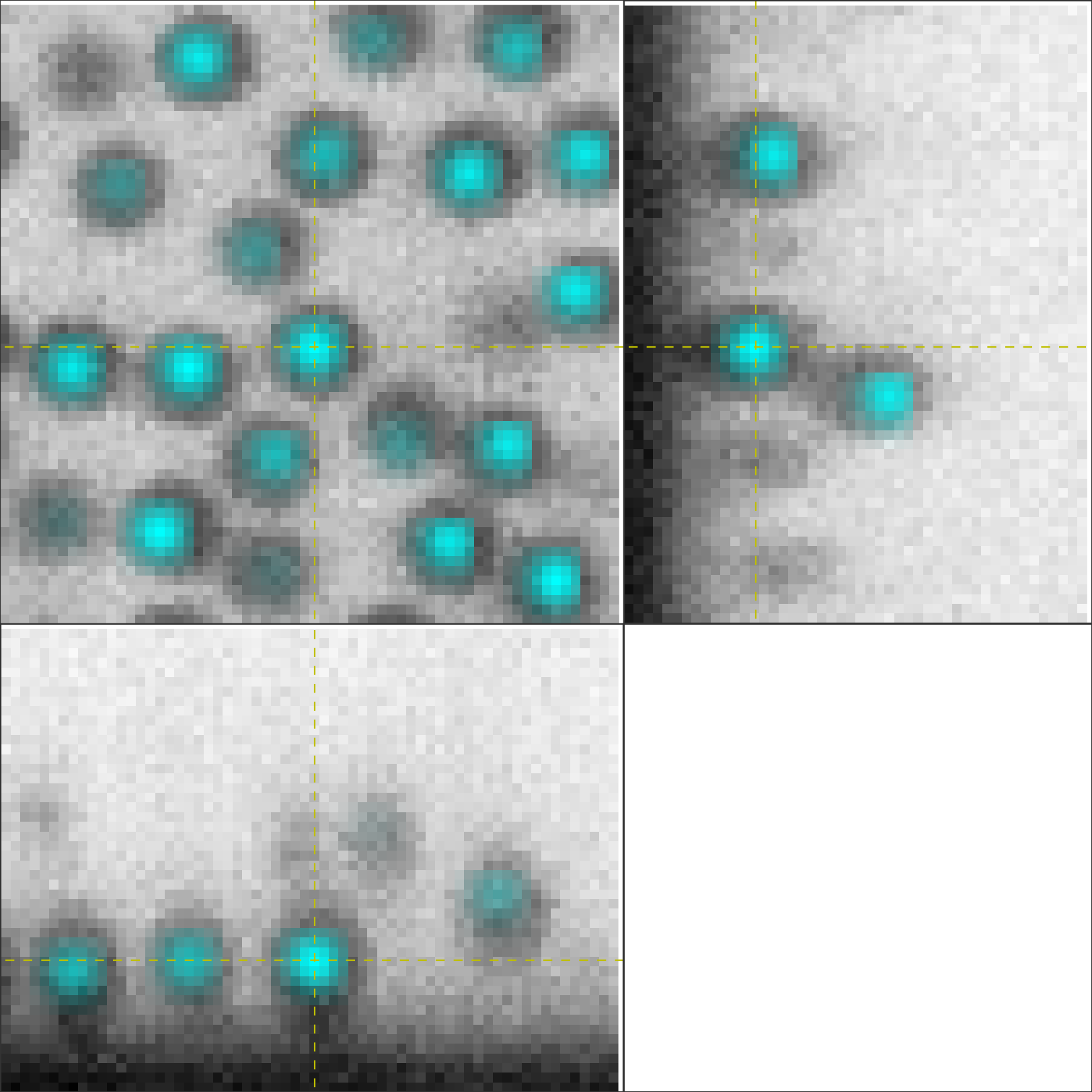
This will pull up an interactive viewer which allows you to examine the raw data, model image, fit residuals, and the different components of the model. Hit Q to cycle through the diffferent view modes, and click on a particular region in the image to see the orthogonal cross-sections of these modes. If you see structure in the residuals of your fit – shadows of particles or stripes and long-wavelength variation in the residuals – then your model isn’t complete or your fit isn’t the best. For my state, we see that the fit is pretty good, as you can see below.

The OrthoManipulator. You can see the raw data on the left and the fit residuals on the right. The residuals are almost perfect Gaussian white noise.

You can look closer for structure in the residuals by looking at the Fourier transform of the residuals (hit W). Again, if you see structure in the residuals in Fourier space, your model isn’t complete or your fit isn’t the best.

If the residuals look OK by eye, check their distribution and deviation from gaussianity. You can do this quickly with

from peri.viz import plots
plots.examine_unexplained_noise(st)

This will bring up a figure that plots the distribution of residuals in real and Fourier space and compares them with a normal distribution expected from the variance of the residuals. If you see significant deviation of the data from a Gaussian, then your model isn’t complete or your fit isn’t good.

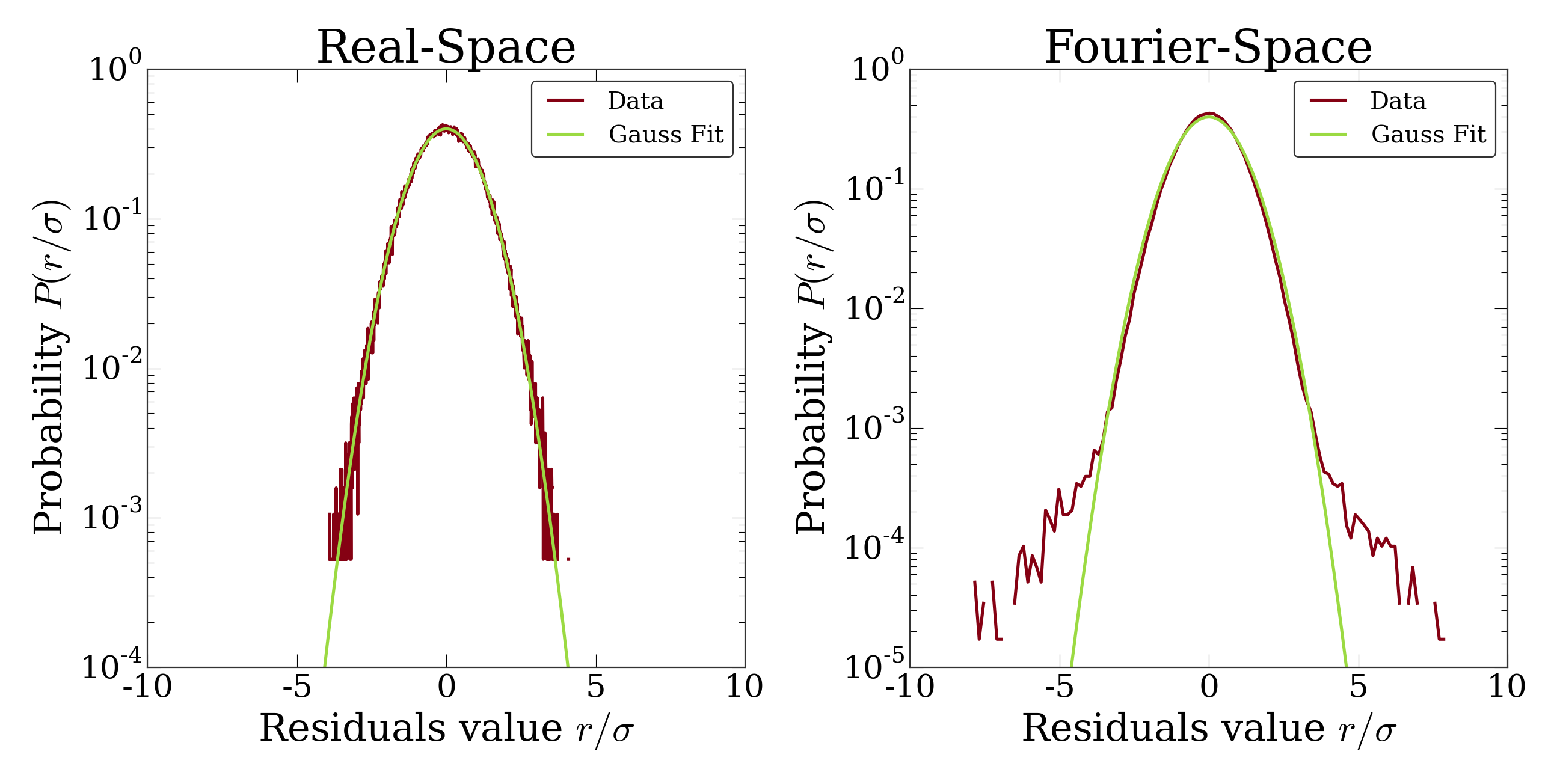
The distribution of residuals in real and Fourier space. They should be perfect Gaussians. While the distribution of real-space residuals is an amazingly perfect Gaussian, there are some deviations in Fourier space at large \(x/\sigma\). Looking at the OrthoManipulator, these arise from a combination of scanning noise on our detector (some lines at \(q_x=0, q_z=0\)) and from incompleteness in our model (a faint ring at moderate \(q\) values).

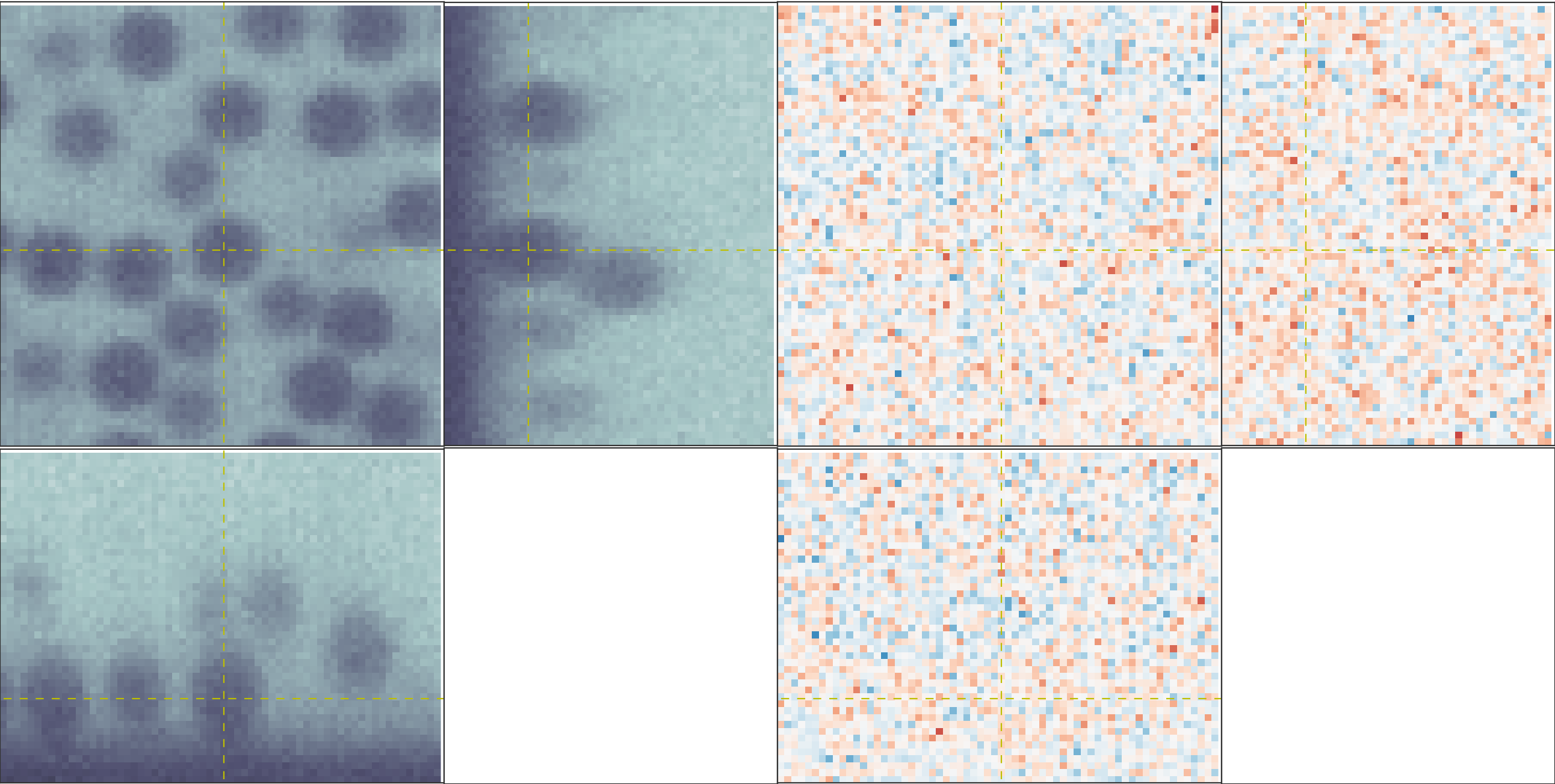
The figure below shows an example of a poorly-fit state. The left panel shows a slice of the residuals from state analyzed above, Since this state is optimized with a near-complete generative model, the residuals in real space (top) look like perfect Gaussian white noise. In Fourier space (bottom), there is some slight structure – probably a result of an incomplete description of our microscope’s actual point-spread function. The center and right panels show the same image fit with an incorrect PSF (an anisotropic Gaussian) and an incomplete ILM (constant illumination and background). For these states, structure is clearly visible in the residuals in both real- and Fourier- space. If your fitted state looks like either of these, then your model is incomplete.

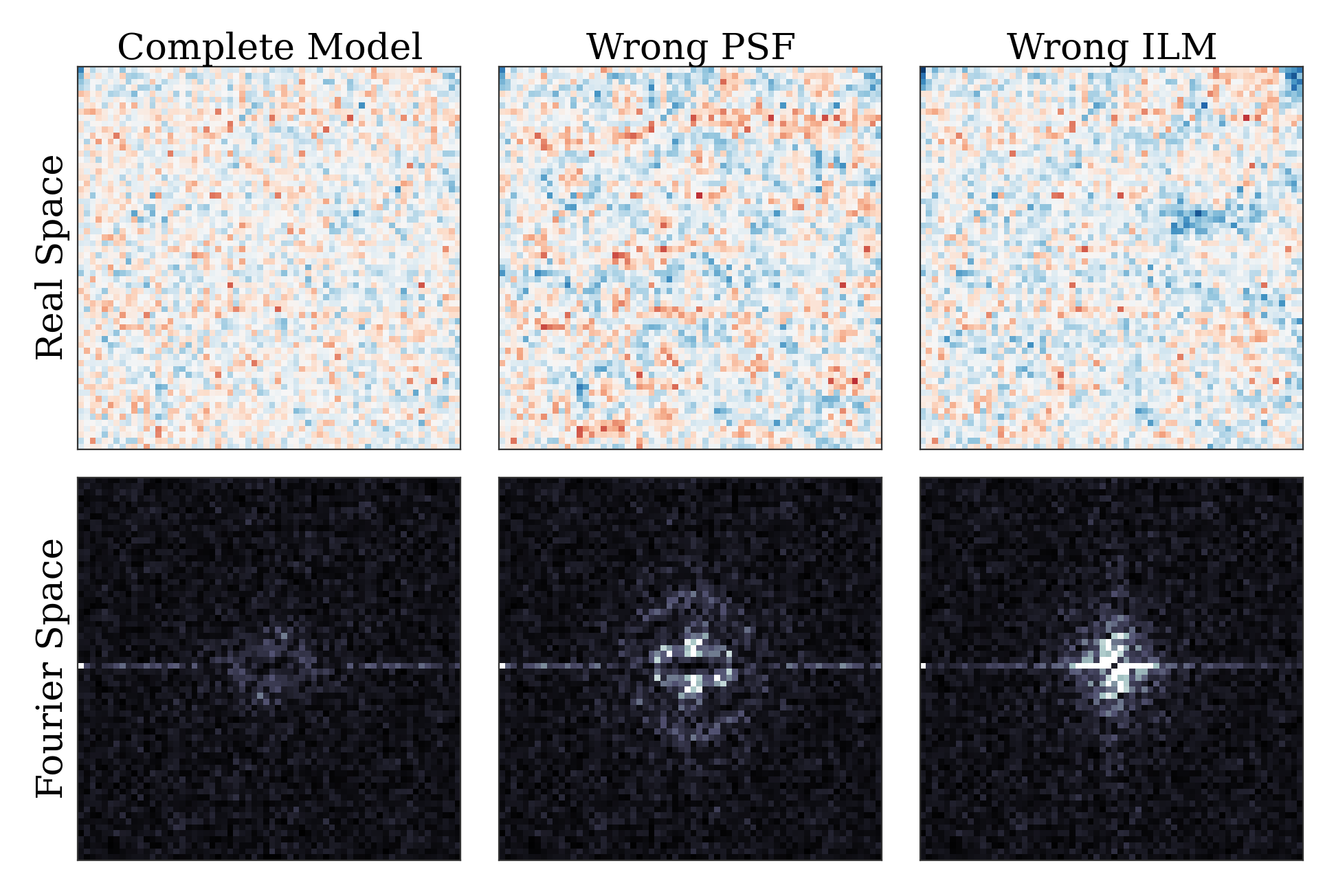
An image fit with a complete model (left) and two incomplete models – one with an insufficiently complex point-spread function (center) and one with an insufficiently complex illumination (right). The states fit with an incorrect model show clear structure in the residuals. The residuals for the incomplete PSF state show clear rings around particles. The residuals for the incomplete ILM state show a slight variation across the image, and also show rings around the particles, as the particles are fit to biased radii to partially compensate for the incomplete ILM. The line of bright pixels at \(q_y=0\) and large \(q_x\) visible in all the Fourier space images are from scan noise in our confocal’s line CCD.

What should you do if the fit is bad? First, I would try more optimizations of the state. If you optimize the state and the error changes, then you weren’t at the best-fit. Keep optimizing until the error stops changing and check again.

If the error doesn’t decrease on optimization and the fit still isn’t good, then your model is incomplete. There are a few possibilities for an incomplete model: (a) you’ve picked the right component, but with the wrong parameters or amount of parameters, (b) you’ve picked the wrong component, (c) the mathematical relationship between the components is incorrect.

Fixing (a) is easy. If you’ve realized that, say, your illumination isn’t high enough order, then just type something like this:

old_ilm = st.get('ilm')
new_ilm = ilms.BarnesStreakLegPoly2P1D(npts=(50,40,20, 20, 20), zorder=7)  # or whatever works
st.set('ilm', new_ilm)

You’ll then need to re-optimize the state all over again. For some components like the illumination and background, you can speed this up a bit by fitting the new component before you continue optimizing, as described in the section on Optimization:

import peri.opt.optimize as opt
opt.fit_comp(new_ilm, old_ilm)

but you’ll still need to re-optimize the state as before.

Fixing problems (b) and (c) are usually just as easy. Say you realized that your microscope is a point scanner and not a line scanning confocal. Just type:

new_psf = exactpsf.FixedSSChebPinholePSF()
st.set('psf', new_psf)

Likewise, say you used the wrong model. (Perhaps your particles are dyed and not the fluid.) Type

new_model = models.ConfocalDyedParticlesModel()  # or whatever model is best
st.set_model(new_model)

Again, you’ll need to re-optimize your state. You might be able to speed the second optimization up by optimizing certain parts first; see the Optimization section for how to do this.

Sometimes, however, the component or model you need isn’t included in the peri package. For instance, you could be imaging rods on a 4Pi microscope or with STEM, changing your objects, point-spread function and image formation model to things that aren’t currently included in the peri package. If this is the case, you’ll need to develop peri to include a new model or component! See the developer’s section of the documentation to get started.

The quality of the data analysis that peri returns is directly related to the quality of the generative model that you use. If your model is not a good description of the data, then the parameters extracted from the model won’t be accurate. Thus it’s very important to ensure that your model accurately describes your experimental images. To ensure that the model is accurate, we’ve found that it’s best to construct the model in a systematic way. For instance, for our confocal images we started by taking a blank image with the laser off, as a way to measure our background intensity. Next we measure and fit an image of just fluorescent dye, to describe our illumination correctly. Then we add a slab, then particles. We’ve provided a stripped-down version of this as a demo in scripts/test_genmodel.py. You should follow a similar protocol for your image formation model.

If the fit is good, use the extracted information from the fit.¶

The ImageState contains all the fitted parameters from the image and their values. The parameters are named with human-readable names that describe briefly which component and/or what the parameter describes.

You can get the parameters and values by typing

print st.params
print st.values

which will print a very long list of all the state’s parameters and values. Usually this isn’t the best format to access the data. Instead, if you want a set of values for a certain set of parameters, use the get_values method. For instance, if I want to know the radius a of the 13th sphere or the fitted wavelength of the laser light from the point-spread function, I can type:

print st.get_values('sph-13-a')  # 13th particle's radius, counting from 0
print st.get_values('psf-laser-wavelength')  # psf's fitted laser wavelength

In addition, there are several convenience functions. You can get all the positions or radii of all the particles in the state through these commands:

pos = st.obj_get_positions()
rad = st.obj_get_radii()

These will return information on all the particles in the state, including ones fit to be outside the image! You can select only the particles inside an image by using peri.test.analyze.good_particles(), which will return a Boolean mask that is True for particles inside the image and False for those outside. The analyze module has many other useful things for analyzing data, such as ways to calculate the packing fraction of the state and ways to save and load states as rapidly-loadable json files.

Making this faster¶

Now that we have a completely-featured image, there is no point in repeating the tedium above to find the best positions and radii for the next image in your data. You can shortcut a lot of the human time by using some of the convenience functions in peri.runner.

All of these runner functions allow you to select the images and previously-featured states interactively through dialog boxes, for convenience. If this is not convenient you can instead pass the filenames for the states and images directly to the runner functions, along with a whole lot more options. Read the documentation if you want to know more!

Here’s how to feature an image quickly…

…using the microscope parameters from another state¶

You’ve already featured a few images from your dataset and have a good peri state for your microscope. You don’t want to spend a ton of time re-featuring the microscope parameters again; you just want the positions in the next image. If the particles in the new image have a radius of roughly 5 pixels, run

runner.get_particles_featuring(5)

This will pull up a file dialog box asking you to select the image to feature and the previously-featured state to take the microscope parameters from. Once you’ve done this, it will run on its own and save the state to the same directory as the image.

…using the microscope parameters and positions from another state¶

If the particles haven’t moved by a whole lot from one frame in your dataset to the next, then you can use

runner.translate_featuring()

which also allows for you to select the image through dialog boxes.

…from scratch¶

The runner functions also allow for featuring images from scratch, without having a previously featured state. However, you’ll need to write and supply a statemaker function that makes a complete ImageState. The statemaker function needs to provide a model that can accurately describe your microscope image formation. See the runner documentation or the example statemaker in scripts/statemaker_example.py. for details. To feature an image of dark spherical particles with a radius of roughly 5 pixels on a bright background, type:

runner.get_initial_featuring(statemaker, 5)

where statemaker is the statemaker function. You’ll select the image through dialog boxes.

…from a guess of positions and radii¶

Perhaps you’ve already spent a lot of time with another method and have a pretty good guess for all the particle positions and radii. In that case, run

runner.feature_from_pos_rad(statemaker, pos, rad)

Once again, you’ll need a statemaker function. You will be able to select the image through dialog boxes.

Using a smaller image¶

As you’ve probably noticed, fitting a complete generative model to a real image takes some time. You can avoid wasting time by starting with a small section of a microscope image, to get an idea of how complete your model is and how many parameters you should include. You can either use a separate small image, or you set the Tile of the image:

from peri.util import Tile, RawImage
tile = Tile([30, 30, 30])  # pixels 0-29 of the image in z,y,x
small_im = RawImage('filename.tif', tile=tile)
# ..and create the ImageState again from scratch as before:
# st = states.ImageState(small_im, [objects, illumination, background,
#        point_spread_function, offset], mdl=model)

If you already had a state, you could then set the new image with s.set_image(im). Alternatively, you can set the image tile directly with the runner functions:

tile = Tile([30, 30, 30])
runner.get_initial_featuring(statemaker, 5, tile=tile)

Checking your model even more¶

Once you have multiple images featured, you can check the quality of your model even more by looking at the variation of parameters from image to image. If your model is truly exact and you are truly at the best-possible fit, then the fitted parameters shouldn’t change from image to image except for the tiny amount of the Cramer-Rao bound. However, if your model is incomplete, the systematic effects missing from the model will couple to the effects included in the model, and small changes in the image (e.g. particles shifting) will cause changes in the fitted parameters abover the Cramer-Rao bound. For our confocal images of spheres, we’ve found that checking the radii variation from frame-to-frame in a movie of freely-diffusing particles is a stringent test of the quality of the fit and model. This is implemented in peri.test.track.calculate_state_radii_fluctuations(), which uses the trackpy package.